Coursera Data Science Specialization: Statistical Inference Course Project part 1


Part 1 of my Statistical Inference project, part of the Johns Hopkins Data Science Specialization on Coursera.
You can find the .Rmd (R Markdown) format here, the html result here and the Rpubs pubblication here.
Statistical Inference Course Project Part 1: Simulation
Massimiliano Figini
October 9, 2016
Investigation of the exponential distribution in R and comparation with the Central Limit Theorem.
Instruction:
1) 1000 Simulation
2) 40 exponentials
3) Lambda = 0.2
# Basic settings
knitr::opts_chunk$set(echo = TRUE,tidy.opts=list(width.cutoff=60),tidy=TRUE)
set.seed(1983)
# Main variables
Lambda = 0.2
Simulation <- NULL
for (i in 1 : 1000) Simulation = c(Simulation, mean(rexp(40,Lambda)))
QUESTION 1: Show the sample mean and compare it to the theoretical mean of the distribution.
Theoretical mean is 1/Lambda, sample mean is the mean of the simulation values.
TheoreticalMean <- 1/Lambda
SampleMean <- mean(Simulation)
paste("Theoretical mean is", round(TheoreticalMean, 3), "sample mean is",
    round(SampleMean, 3))
## [1] "Theoretical mean is 5 sample mean is 5.028"
The sample mean is very close to the theoretical mean.
QUESTION 2: Show how variable the sample is (via variance) and compare it to the theoretical variance of the distribution.
I can calculate theoretical variance by dividing 1/Lambda for the square root of the number of exponenentials and squaring all.
TheoreticalVariance <- ((1/Lambda)/sqrt(40))^2
SampleVariance <- var(Simulation)
paste("Theoretical variance is", TheoreticalVariance, "sample variance is",
    round(SampleVariance, 3))
## [1] "Theoretical variance is 0.625 sample variance is 0.617"
The sample variance is very close to the theoretical variance.
QUESTION 3: Show that the distribution is approximately normal.
Using an histogram I can easily see if the distribution is approximately normal.
hist(Simulation, probability = TRUE, breaks = 40, col = "red",
    main = "Distribution", xlab = "Simulation means")
lines(density(Simulation), lwd = 3, col = "black")
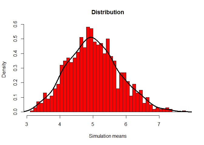
The distribution of averages of random sampled exponentials is like a normal distribution.